


At Alectio, we’re usually known to help ML teams reduce the size of their datasets; our typical users come to us when they have more data than they know what to do with, and when training on their entire dataset is just not feasible, the reason being that most people associate Active Learning (which is at the core of our platform) with reduction of labeling costs.
However, we know that Active Learning has many more applications, and can in fact, be just as helpful when you’re dealing with a small dataset. That’s because the smaller the dataset, the more vulnerable you are to “data poisoning”; in other terms, you can get away with a small dataset, but only if the data is very clean and perfectly annotated.
Showing you how you can train a better model with a tiny dataset using an Active Learning-based approach is what the blog post is all about, so keep on reading!
About the dataset:
Since a lot of the work on data curation out there usually revolves around Computer Vision, we have decided to add an additional twist here and work on a slightly different use case: that of Mental Health, which is also extremely timely in those post-pandemic times.
The dataset is essentially a collection of sensor data retrieved from patients suffering from depression. It contains activity recordings of 23 patients, suffering from unipolar and bipolar depression, and 32 healthy persons. The dataset is labeled by the medical experts on the Montgomery-Asberg Depression Rating Scale (MADRS).
The actigraph devices were used to record the data and a total of 693 days were collected. 402 of these days were collected for the control or the healthy class and the remaining were recorded for the conditioned class.
For each patient, a csv file containing the actigraph data collected over time is provided. Along with the activity recordings, the MADRS scores are also provided. Other information such as gender, type of depression, education, marriage, and work are provided about the patient.
Application of the dataset:
Considering each day as an individual datapoint, we aim to classify it into depressed or non-depressed classes. Using different query strategies, we aim to resolve the imbalanced nature of this dataset.
Feature extraction:
In order to use sklearn models, we have extracted certain features from the activity recordings such as mean activity level, corresponding standard deviation and percentage of events with no activity i.e. activity level=0.
Analysis:


This image shows that approximately 2/3rd of the dataset is for the normal class. Hence, we are dealing with an imbalanced dataset. Such datasets are usually modeled with solutions like SMOTE, majority undersampling (if you are unfamiliar with the topic, we suggest you start here).
However, in our case, we want to evaluate the capabilities of Active Learning as an in-training undersampling engine and simply let the query strategy decide what samples are required to train the model better with fewer samples. This approach also offers a particularly interesting benefit: with Active Learning, we do not require to:
- have the data annotated before hand (knowledge of the ground truth is a fairly common prerequisite to rebalancing, and,
- look at the training data itself (non-intrusiveness is pretty useful when you work with sensitive data that users don’t want to share).
Results and takeaways:
Now, the fact that Active Learning offers so many advantages (I mean, did you ever think of Active Learning as a way to rebalance your dataset?), doesn’t mean it’s easy, and we’ve explained why before. Getting an Active Learning process right requires a lot of tuning – even more so if you’re new to it. That’s because most people who’ve heard about Active Learning before believe it can be reduced to uncertainty-based querying strategies, when in reality, there are countless ways and types of strategies. Active Learning is really just an incremental learning paradigm where you use the information you have at a specific point in time to “guide” the selection of the next batch (called a loop) of data. The way the guiding happens is really up to the ML scientists using it.

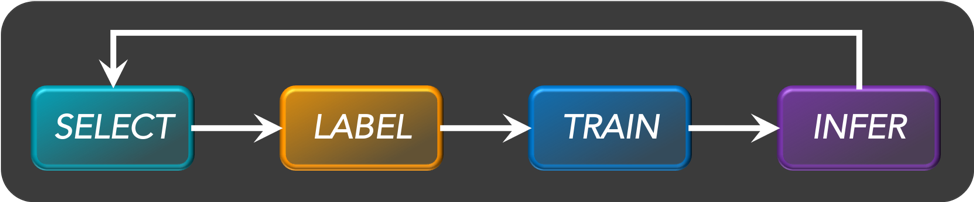
Figure 1: The flow of an active learning process. The secret is in implementing the best algorithm possible for the SELECT step, which can really be anything.
Analyzing the performance of our Auto Active Learning algorithm
Our “secret sauce” is in the algorithms we use for the selection step. While we can’t disclose everything, we can say though that that SELECT step can be ‘smart’ (i.e., it can be an ML model instead of a brute-force, arbitrary sampling function), and that there is no reason why that function wouldn’t evolve over loops (and over time).
One of our most successful algorithms is one we named ‘Auto Active Learning’, which we’ve decided to compare against some of the most common “vanilla” selection strategies.

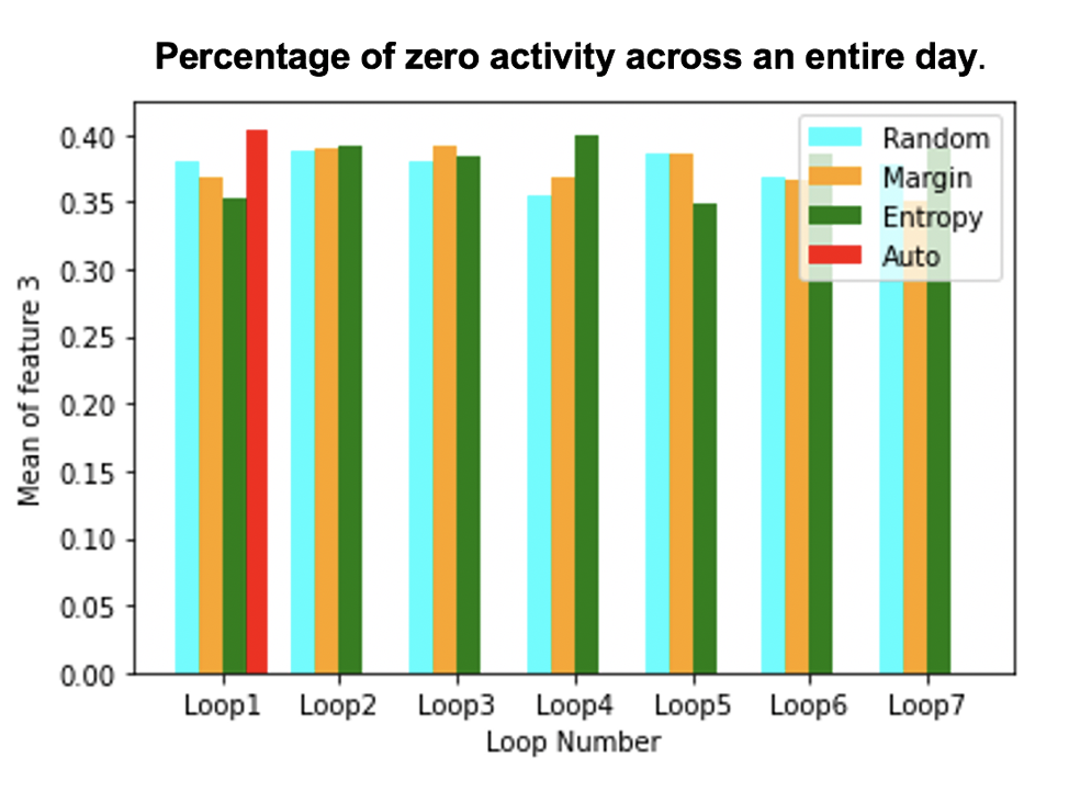
Figure 2: Looking at the evolution of one of the key features across Active Learning loops is one way to gain visibility into what is useful to the learning process.
Now, another facet of Active Learning is that: while we are using it as a real-time data selection process, we can also use it as an explainability tool to identify what data is most informative to the model, and attempt to understand why.
Take a look at Figure 2; the graph shows the mean of one of the features for the samples selected across loops with different query strategies. That feature represents the percentage of inactive periods throughout an entire day for a patient, which a mental health expert could certainly confirm is extremely important in the prediction.
And what we observe here, is that our Auto Active Learning strategy prioritized data from ‘inactive’ patients at an early stage (loop 1 is the first “smart” loop; we usually refer to the random initialization loop as loop 0, and it’s not represented here), before zeroing on active patients. For example, the process selects 24 samples for loop 3. Each of these selected samples are from the depression class, which is the minority one – and they got selected without any knowledge of the class that they belonged to.

It’s also interesting to note that the increase in the accuracy curve from 2nd loop to 3rd loop is quite significant in the Auto Active Learning learning curve. Hence, this strategy is able to identify unique samples in the entire dataset and help to achieve better model performances faster with significantly less samples.

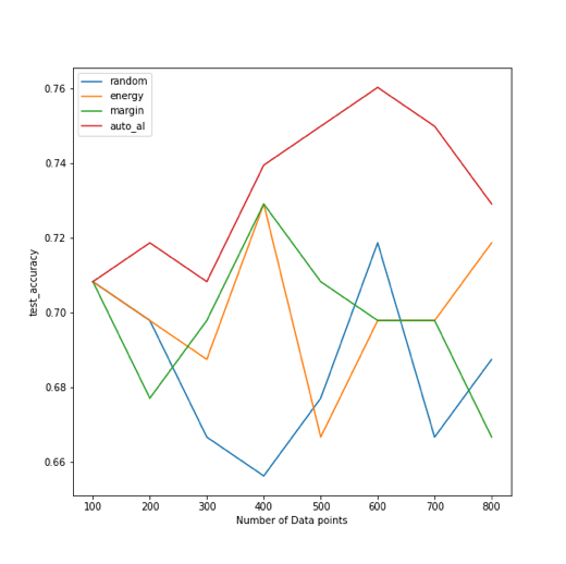
Figure 4: Comparing the learning curves of multiple curation experiments, ran with various querying strategies. Choosing your querying strategy wisely is critical – but it’s not easy!
We can conclude that Auto Active Learning is capable of strategically guiding the model’s learning process. But that’s not all; we did it all without actually looking at the data since this is just a post-analysis; Auto Active Learning did operate some sophisticated rebalancing of the data to boost the learning process – and we gained some understanding of the relationship between the model and the data as a bonus!
Note also that the last loops of the Auto Active Learning process actually cause a reduction of the performance of the model (meaning the remaining data is harmful to the model). Ultimately, we reach the optimal model performance with 75% of the dataset AND an accuracy several points higher (at close to 76%) than the results obtained when training on the entire dataset (69.7%). What not to love?
Analysis of the ‘random query’ across loops:
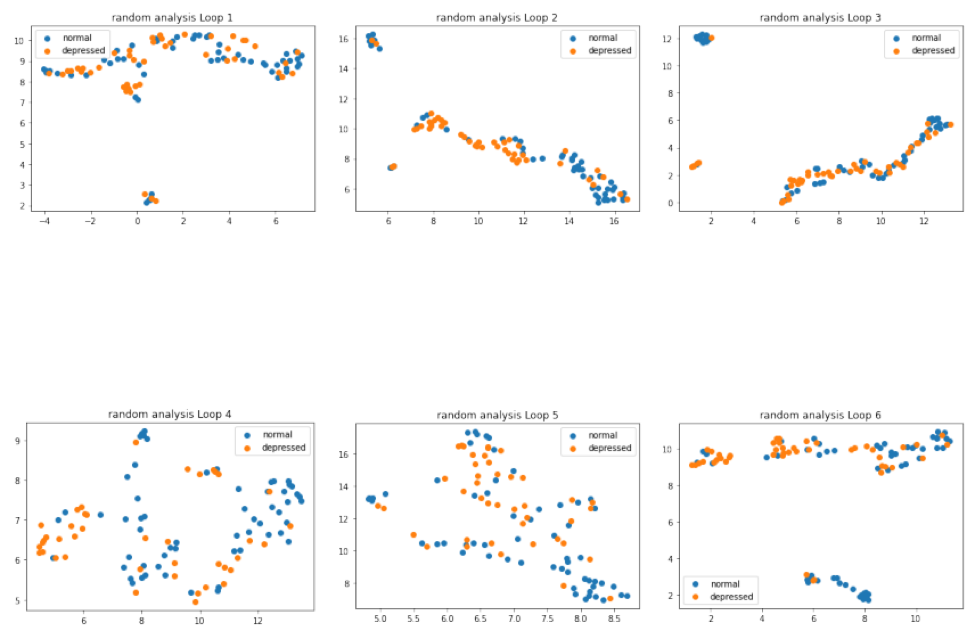

Each graph in the above graph is the UMAP representation of data selected in that loop by the random query strategy. As seen in the above graphs, loop numbers 2,3 and 6 have samples selected which are very difficult to separate into normal and depressed classes. Yet samples which are selected in the loop 4 and 5 are very easy to be separated and a decision boundary can be defined. This behaviour can be easily mapped onto the learning curve for the random query strategy. In other terms, the model learns when the process selects well separated samples by chance.
Thus, random selection of the samples is not necessarily helping the model’s learning process; in fact, it can even hurt the overall accuracy on top of increasing the cost of the labeling for the dataset. Definitely a lose-lose situation!
Conclusion
If you started with the belief that Active Learning can’t help if your dataset is small, we hope that we have been able to change your mind. We’ve covered here a few of the different, misunderstood applications of Active Learning:
- Active Learning can help curate a dataset, no matter its size
- Active Learning is not just useful to save on data labeling (though in such a use case, the ground truth label is essentially the diagnostic of psychiatrist, and hence can be very expensive to acquire), but also to boost model performance
- Active Learning can also be used as an analytical and even an explainability tool
This is just a fraction of what data curation can do for you. Contact us if you want to learn more and book your Alectio demo today!