
We tried to ‘lie’ to our classification model by feeding mis-labeled data and analyzed the results…
[This article has been coauthored by Jennifer Prendki and Akanksha Devkar from Alectio, and has been published in Analytics Vidhya]
Data scientists, have you ever wondered how many classes you should use when working on a classification problem? If so, you are not alone. Of course, often times, the number of classes is dictated by the business problem you are trying to solve, and that’s not really up to you. And in that case, no doubt that an important question kept nagging you: what if I don’t have the data for that? There are, in fact, many reasons why your data would actually not support your use case; just to name a few:
- The class imbalance in your training set,
- The underrepresentation of each class: too many classes for too little data would lead to a case where there wouldn’t be enough examples for a model to learn each class,
- Class “specificity*”: the more alike two classes, the easier it would be to mistake one for the other; for example, it is easier to mistake a Labrador for a Golden Retriever than a dog for a cat.
That is a lot to consider even before building a model; and the truth is, your endeavors might be doomed from the beginning, no matter how hard you try to get a high performance model, either because your data quality is really subpar, or because you don’t have enough of it to allow your model to learn. That’s when we realized that there was in fact no good framework to identify how well separated two classes were, or how suitable a dataset was to learn how to differentiate examples from two different classes. And that’s what we set out to fix.
Intuitively, the success of a classification project depends a lot on how well separated classes are; the least “grey areas”, the better. Clearly differentiated classes don’t leave a lot of opportunities for any model to mix things up because the features learnt for each class will be specific to each one of them.
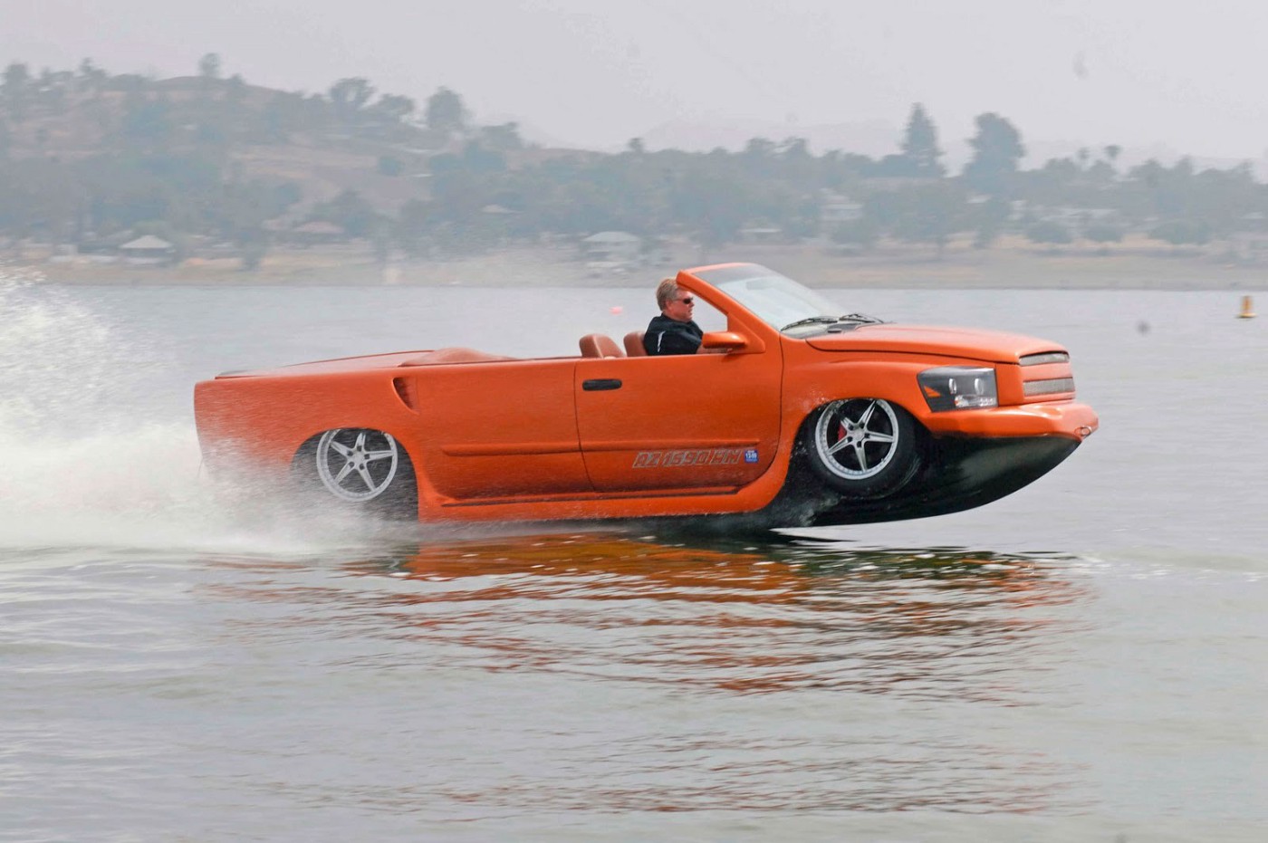
Figure 1: An example of confusing image: should this image be classified as a car or a boat?
Things get more complicated when “look-alike” classes appear, or, for example, when items can classify as more than one type of object. It is in this spirit of discovering a process to measure “look-alikeness” that we started this study on CIFAR-10 with a small custom deep neural net. The underlying idea is actually pretty simple: to find out which classes are easy for a model to confuse, just try confusing the model and see how easily it gets fooled.
Experiment 1: Labeling Noise Induction
For the purpose of observing effects of labeling noise induction, we took the clean CIFAR-10 and voluntarily injected labeling noise in the training set’s ground truth labels. The process is explained as below:
- Randomly select x% of the training set,
- Randomly shuffle the labels for those selected records; call this sample Sx,
- Train the same model using S_x; here, our model is a small (6-layer) CNN (non-important for the conclusion of our experiments),
- Analyze the confusion matrix.
Of course, because some variance would be expected from selecting such a sample randomly, we repeated the same experiment multiple times (5 [five] times, due to our own resource limitations) for each amount of pollution and averaged the results before drawing any conclusions. Below, we show the results for the baseline (trained on the entire training set, S_0%) and the average confusion matrix for S_10%, i, 1≲i≲5.
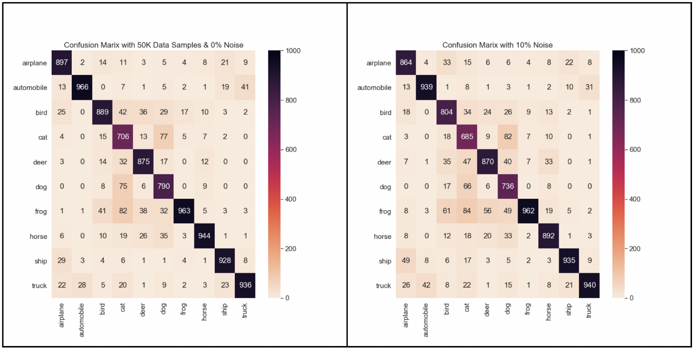
Figure 2: The confusion matrix on the left shows the confusion matrix obtained when training with the full CIFAR-10 dataset; on the right is the average confusion matrix when 10% of the data is mislabeled.
Important note: the ground truth labels are read at the bottom and the predicted labels on the left (so that on the baseline, there are 82 real cats that were predicted as frogs). We will use the same convention in the rest of the post.
First analysis
A very first finding is that even for the baseline, the confusion matrix isn’t symmetrical. Not much surprise here, but it is worth noting that there is directionality involved here: it’s easier for instance for this specific model to mistake a ‘cat’ for ‘deer’, than ‘deer’ for ‘cat’, which means that it is not possible to define a “distance” in the mathematical sense of the term (since distances are symmetrical) between two classes.
We can also see that the accuracy for airplanes isn’t affected much by the pollution; interestingly, injecting random labeling noise seems to decrease the confusion of ‘cat’ as ‘dog’ while increasing the confusion ‘dog’ as ‘frog’, indicating that noise benefits generalization.
Conclusions:
- Not all classes are equally resistant to labeling noise.
- Cross-class confusion is directional.
To allow you to gain some intuition into wrong predictions, some ‘cat’ class images that were identified as ‘frog’ class along with the probability for that prediction with 10% random pollution injected in the training data are shown in Figure 3.
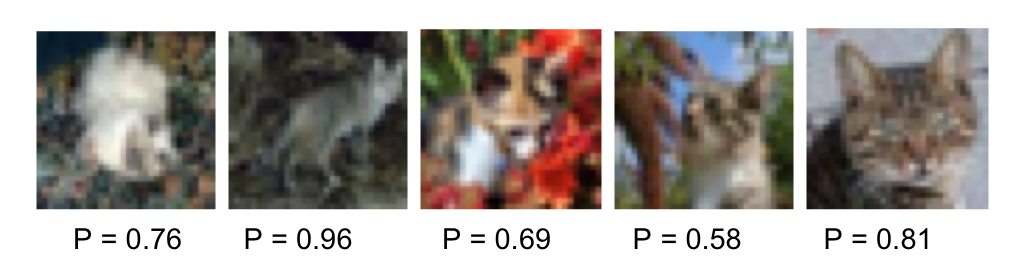
Figure 3: Images of cats mistaken as frogs. The numbers underneath represent the confidence levels with which they were respectively predicted. The higher the confidence level, the more ‘convinced’ the model is that it made the right prediction.
Taking the labeling noise induction further
Let’s keep increasing the amount of labeling pollution, knowing that in real life, a higher pollution rate would be the consequence of poorer labeling accuracy (typically, more than one annotation is requested when labeling data in order to limit the impact of labeling voluntary or involuntary mistakes).
After running that experiment, we observe that the ‘cat’ class is systematically the least accurate across all pollution levels; however, in the relative confusion matrix, we see that ‘bird’ class is the most affected one. So even though the ‘cat’ class is the one that makes the least number of correct predictions, the ‘bird’ class is more severely impacted by the induction of labeling pollution (see the details on Figure 4).
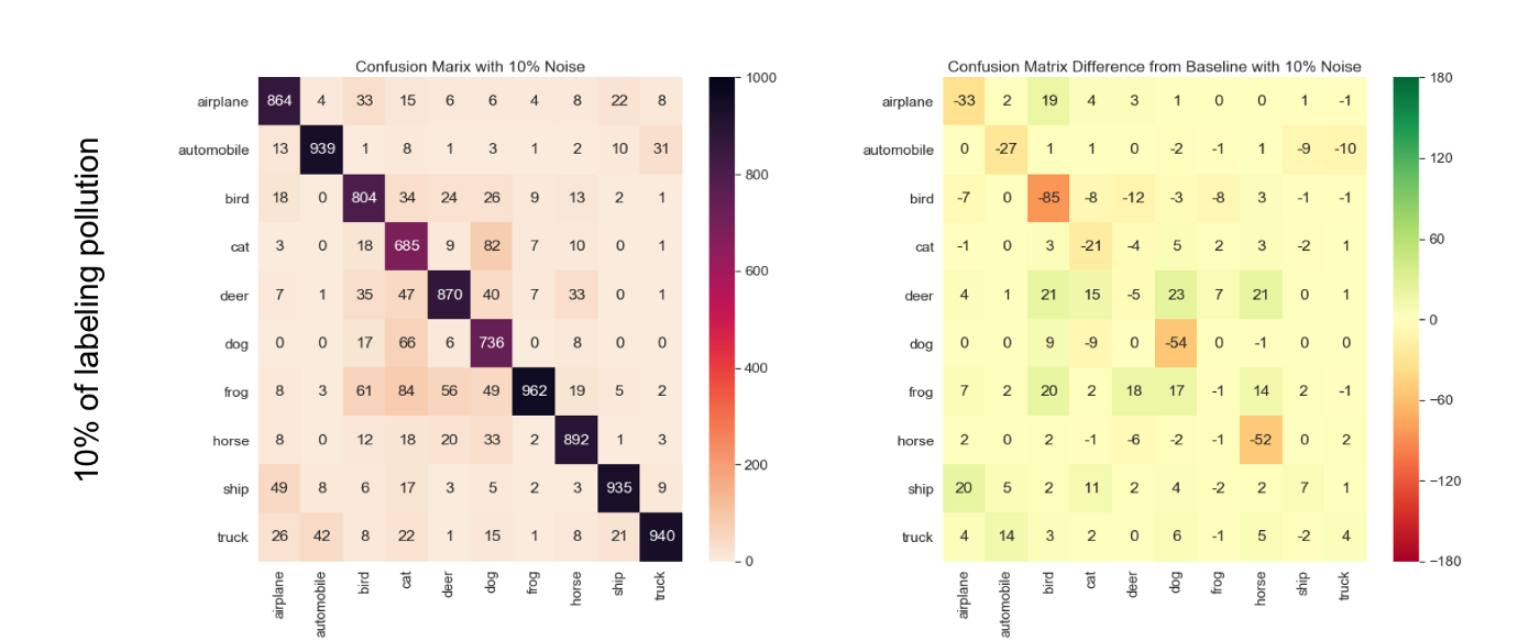
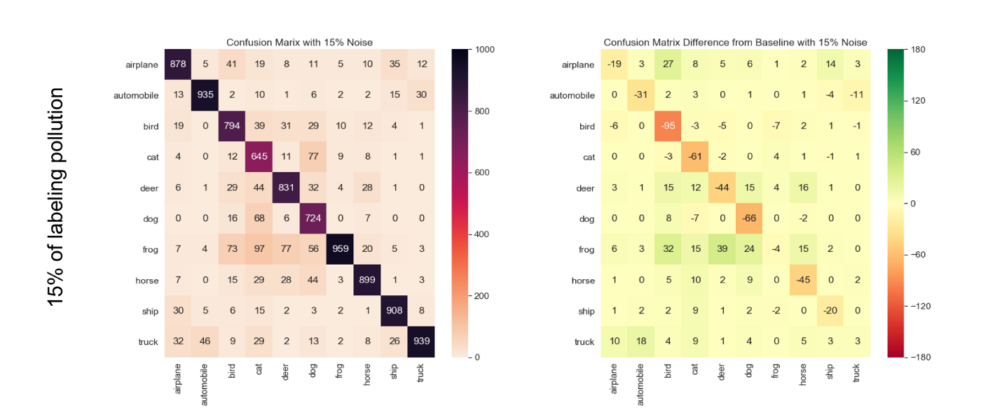

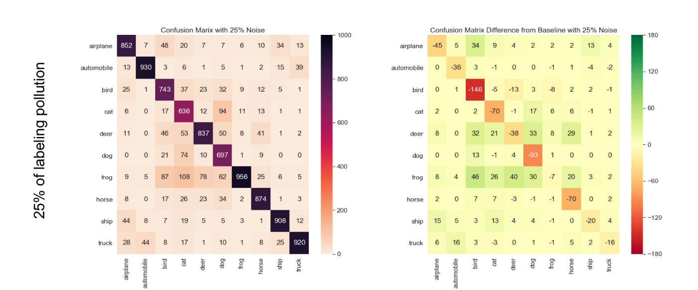
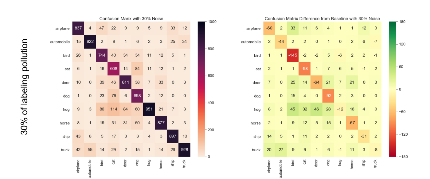 Figure 4: The left column shows confusion matrix for various labeling pollution amounts, while the right column shows relative confusion matrix for the same pollution amount respectively. The left confusion matrices are obtained by averaging the results of 5 runs to smooth out outlier runs; the relative confusion matrix on the right is the difference of that average matrix and the confusion matrix obtained for the baseline run.
Experiment 2: Data Reduction
A fundamental question then arises: if some classes are more impacted than others when we inject noise in our data, is that due to the fact that the model got misled by the wrong labels, or simply from a lower volume of reliable training data? In order to answer that question, after analyzing how labeling noise impacted the different classes in CIFAR-10, we decided to run an additional experiment to evaluate the impact of data volume on accuracy.
In this experiment we went on reducing the size of training set and see the effects on the confusion matrix. Note, that this data reduction experiment was only performed on the clean CIFAR-10, i.e. without any labeling pollution.
From the results displayed on Figure 5, it is worth noting that, for the model we used, we observed just 1% drop in accuracy with a significant 10K data samples drop in training data from the original 50K data samples to 40K data samples.
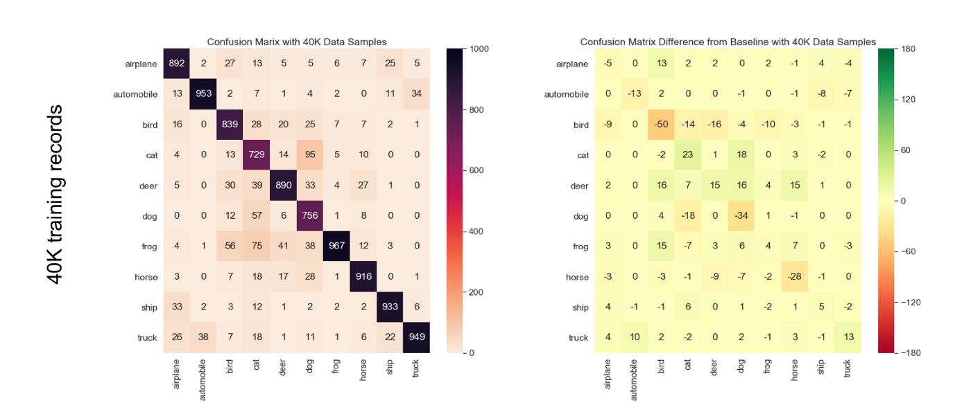

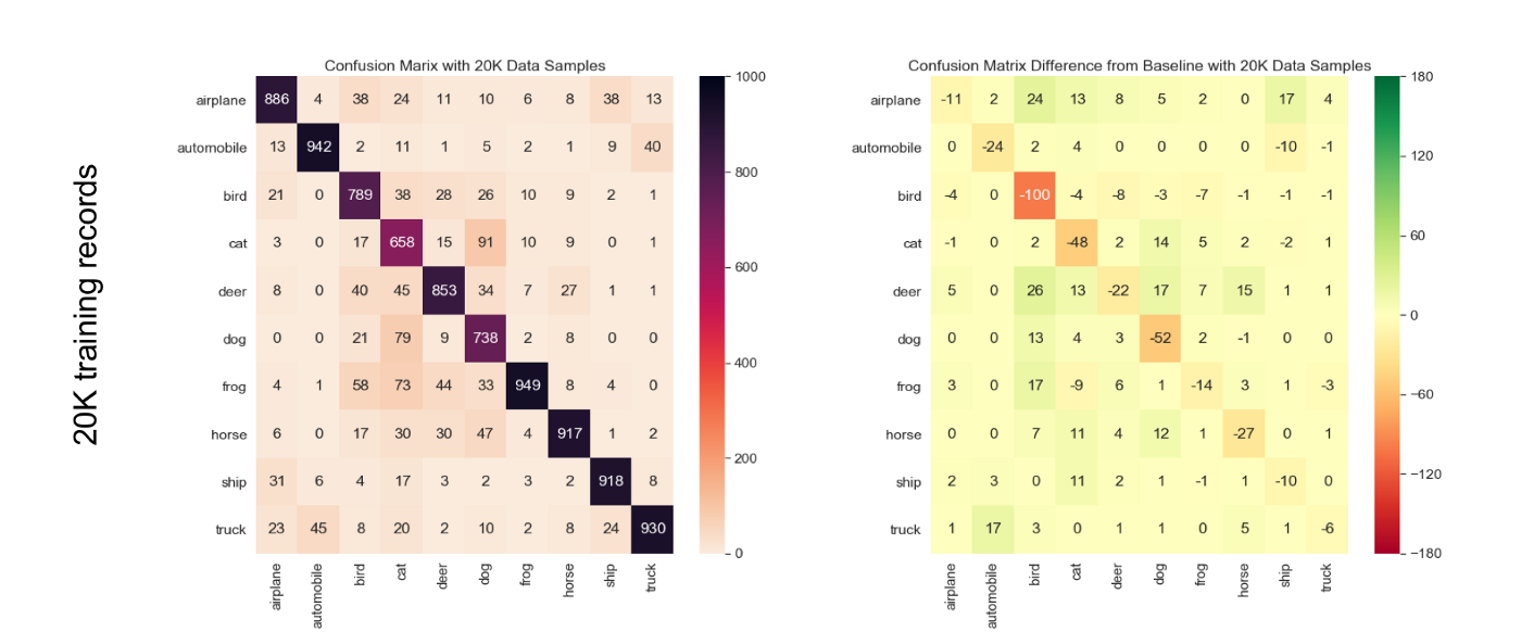
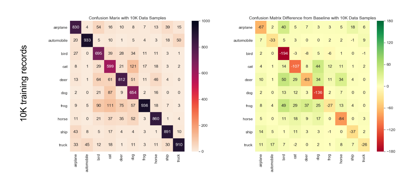
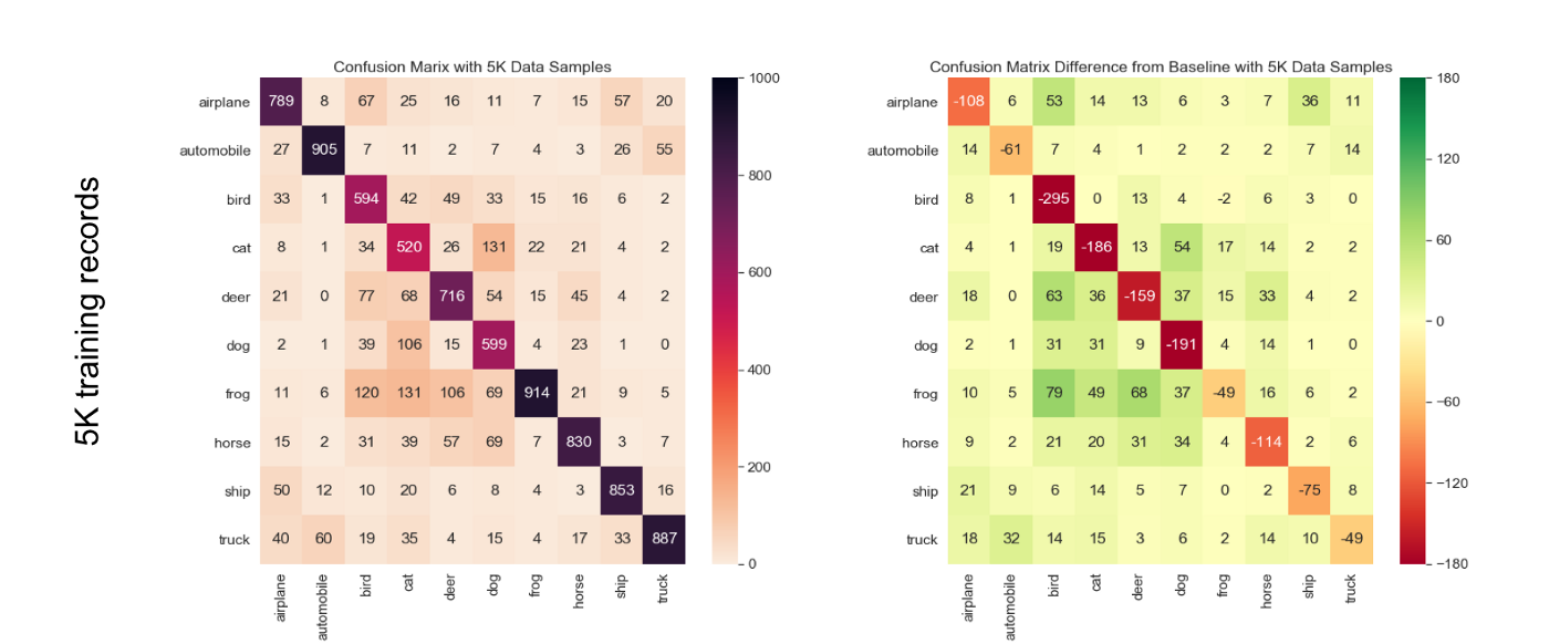 Figure 5: Left column shows confusion matrix for various data volume amounts and right column shows relative confusion matrix for the same number of training examples. The left confusion matrices are obtained by averaging the results of 5 runs to smooth out outlier runs; the relative confusion matrix on the right is the difference of that average matrix and the confusion matrix obtained for the baseline run.
Just like in the case of labeling pollution, the ‘cat’ class is the least accurate in the absolute but the ‘bird’ class is the most relatively sensitive to data reduction. We can see that ‘bird’ class is significantly more impacted than the others, and when reducing the size of the training set by 10K from 50K, the absolute number of additional mistakes made by the model goes up by 50 already.
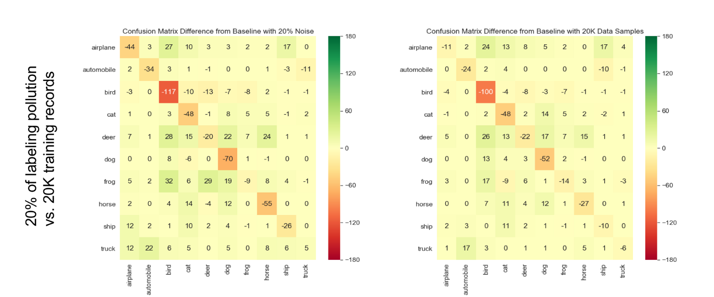
Figure 6: Side-by-side comparison of the relative confusion matrices for the 20% noise induction experiment (left) and the 60% data reduction experiment (right).
In an attempt to compare the relative effect of labeling quality vs. data quantity, we show in Figure 6 the relative confusion matrices for a 20% amount of labeling noise and 60% drop in data volume. While we see that ‘cat’ and ‘deer’ classes are equally impacted in both cases, the ‘airplane’ and ‘horse’ classes are more impacted by labeling noise induction.
Conclusions:
- Data volume reduction and labeling pollution affect different classes in different ways.
- Different classes have a varied response to each effect, and can either be more resistant to labeling noise, or to a reduction in the size of the training set.
One can immediately note that the hottest cell when we start polluting our training set is {bird, bird}; by contrast, the hottest cell for the baseline was {cat, cat}. This means that even if the ‘bird’ class was not the hardest for the model to learn, it is the one that’s taking the biggest hit from labeling pollution and data reduction, and hence, it is the most sensitive to labeling noise. Things even seem to take a turn for the worse somewhere between 15% and 20% of labeling noise; it seems that 20% labeling noise is just too much for the ‘bird’ class to handle. In the meantime, the ‘frog’ and ‘truck’ classes seem particularly stable.
Now, it is a somewhat intuitive result when looking at a sample of the training images in each one of the ‘bird’ and ‘truck’ classes (see Figure 7).
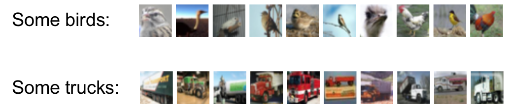
Figure 7: Samples of training images for the ‘bird’ and ‘truck’ classes. We can see a larger ‘variance’ for ‘bird’, which might make it harder for a model to identify common learnable features to generalize what a bird is.
We are zooming into this effect by looking at the {bird, bird} matrix element as a function of the amount of labeling noise used in the training set and amount of data samples used for training.
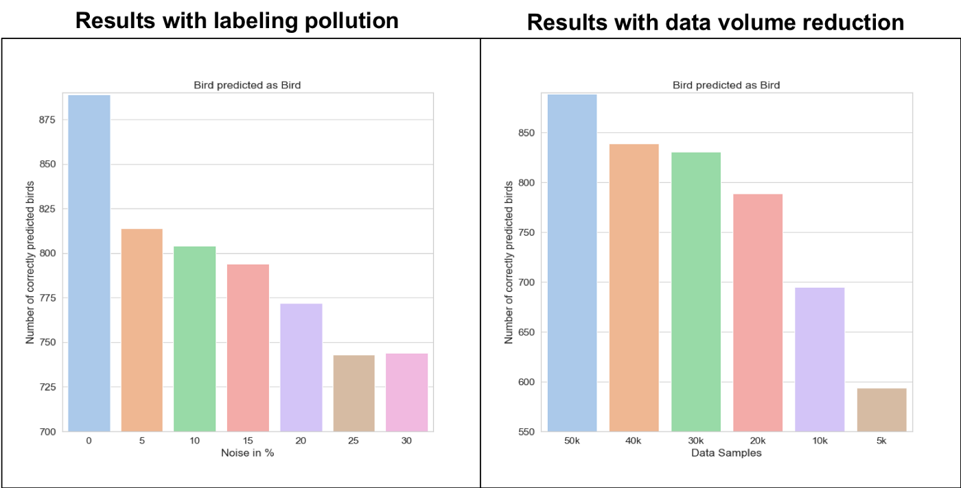
Figure 8: Plot of the value of the {bird, bird} matrix element extracted from the relative confusion matrix with pollution and data reduction.
Conclusions:
- The relationship between amount of labeling noise and the accuracy depends a lot on the class. It is also non-linear.
Putting it together
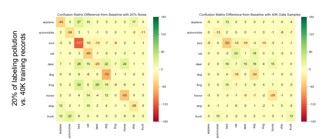
Figure 9: Side-by-side comparison of the relative confusion matrices for the 20% noise induction experiment (left) and the 20% data reduction experiment (right).
Let’s now answer the question we had earlier: do results get worse with labeling noise induction because we reduced the amount of ‘good’ data that the model has to learn from, or because bad labels are misleading the model? By comparing the results for a 20% level of labeling noise and those for a 20% volume reduction, we can see right away that the accuracy is always worse for labeling pollution, proving that bad labels are actually impacting the model negatively even in small quantity.
In an effort to compare how different classes respond to the stress we applied to our model, we present a summary of our various experiments in one single table below, where each column shows the classes sorted by order of accuracy: for the baseline, the class with the worst accuracy was ‘cat’, followed by ‘dog’ and ’deer’. The order is somewhat shuffled from one experiment to the other.
What we see here is that the ‘cat’ class, being the one that performs worse on the baseline, is also the worst with labeling noise induction and data reduction. That suggests that the model we used is not finding it easy to learn what cats are, and gets easily fooled with fake cats as well. The ‘bird’ class is especially badly impacted by both data volume reduction.
By contrast, ‘frog’ and ‘truck’ classes are fairly easy for the model to learn, and “lying” to the model about ‘frog’ and ‘truck’ doesn’t seem to matter much. In that sense, it’s like the ‘frog’ and ‘truck’ class can take significantly more bad labels compared to other classes.
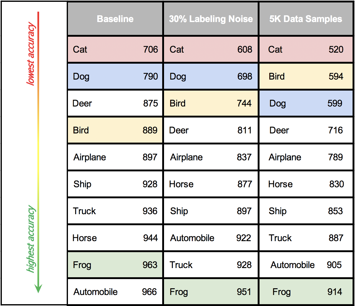
Figure 10: Classes sorted accordingly to their accuracy with their respective true prediction scores, across various experiments (left: baseline, center: 30% labeling noise, right: 90% noise reduction). We can immediately see how the ‘bird’ class, which was performing worse than the ‘dog’ class in the baseline, gets worse than ‘dog’ with extreme volume reduction.
Final conclusions
A single look at the confusion matrix on our baseline model showed that some classes were more easily confused for each other; besides, we saw the concept of cross-class confusion was non-directional. Some further experiments proved that even voluntarily trying to confuse the model with bad training labels (i.e.: trying to “lie” to the model) was not equally successful for all classes, and found in the process that some classes were more sensitive to bad labels that others. In other terms, not only are some confusions more likely than others (even on the baseline), but they are also a function of both labeling quality and data quantity (and some confusions become more likely much faster than others when the training data’s volume or quality drops).
Next steps
In future sequels to this blog post, we will discuss:
- Whether cross-class confusion has a dependency on the model used, or if it is intrinsic to the dataset itself.
- Whether/how data quantity can make up for labeling quality.
(*) Here, we don’t mean “specificity” in the Machine Learning sense of the term.
Need help curating your dataset or diagnosing your model? Contact us at Alectio! 🙂


0 Comments